

The Real Numbers
Theorem 5. There exists a real number c for which c2 = 2.
Proof. Define a sequence
![]() of closed intervals in R
recursively as follows. First,
of closed intervals in R
recursively as follows. First,
let

and let
 = the midpoint of
 .
.
Next, let
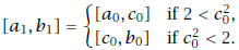
(We cannot have  because no rational number
has square 2.) In general, once
because no rational number
has square 2.) In general, once 
has been constructed, let
 = the midpoint of
and then let
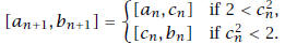
(Since no rational number has square 2, in fact the case
 never arises.)
By the construction, 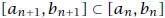 for all n = 0, 1, 2, . . . . Then
for all n = 0, 1, 2, . . . . (Why?)
By the Nested Interval Property of R, there exists some c with
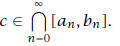
We are going to show that c2 = 2.
Just suppose c2 ≠ 2. Define

so that ε > 0. By the Archimedean Ordering Property of R, there exits a positive
integer n for
which

(Why?)
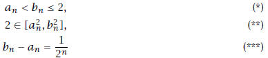
Fix such an n. Since both c2 and 2 are in
 , then
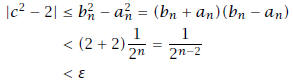
This is impossible because |c2 - 2| = ε.
Exercise 6. Use the method of the preceding proof to establish that
 exists.
Exercise 7. Prove uniqueness of the number c whose existence is guaranteed by
Theorem 5.
The method of proof of Theorem 5 does not merely establish existence of a real
number c
whose square is 2. It also provides a method for approximating that number as
closely as we
wish. Indeed, look again at the construction of the intervals
![]() . The
number c we want
. The
number c we want
belongs to each of these intervals (and is different from the endpoints of
each). Initially, all we
know about c is that 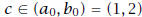 , that is,
1 < c < 2.
If we use the midpoint ![]() = 1.5 as an approximation to c, the the error in that
approximation—
= 1.5 as an approximation to c, the the error in that
approximation—
the size  of the difference between c and the approximation
![]() —satisfies
—satisfies

(half the length of ![]() =
[1, 2]). Next, since
=
[1, 2]). Next, since 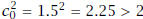 , then
[1, 1.5]. So now we know c ∈ (1, 1.5), that is,
1 < c < 1.5.
If we use the midpoint  as a new approximation to c, then the error
 in this
approximation satisfies
(half the length of  . Next, since
 , then
 . So now we know that c ∈ (1.25, 1.5), that is,
1.25 < c < 1.5.
If we use the midpoint  as a new
approximation to c, then the error
as a new
approximation to c, then the error  in this
approximation satisfies
With each successive bisection of the interval, the number c is trapped inside
an interval of
half the length of the interval used in the previous step, and the error in the
approximating
midpoint is halved. This method is known as the "Bisection Method".
Exercise 8. Continue the Bisection Method begun above so as to approximate
![]() with an error
with an error
less than 0.01.
The method of proof used for Theorem 5—constructing a nested sequence of closed
intervals—
is applicable for the next theorem, too.
Recall the relevant definitions (which we originally gave in N). Let A
 R. An upper bound
of A in R is a number b ∈ R such that a ≤ b for every a ∈ A. The set A is bounded
above in
R when there exists some upper bound of A in R.
About N you proved that each nonempty subset A of N that is bounded above in N
has a
greatest element. Such a greatest element g of A is an upper bound of A in N
that is no greater
than any other upper bound of A in N; in other words, g is the least element of
the set of all
upper bounds of A in N. So this greatest element g of A is least upper bound of
A in N.
A subset of R that is bounded above in R need not have a greatest element. For
example,
the open interval (0, 1) in R has no greatest element (why?). But it does have a
least upper
bound in R, namely, the real number 1. The following theorem generalizes this
example.
Theorem 9 (Order Completeness of R). Each nonempty subset
of R that is bounded above has
a least upper bound.
Proof. See the proof of Theorem 3.3.13. In that proof, just change F to R and
change the term
"supremum" to "least upper bound".