Matrices Overview

Matrices Overview
“Unfortunately, no one can be told what the Matrix is. You have to see it for yourself.”
Morpheus – The Matrix (1999)

Well, I’ll do my best to explain it…

A Matrix is a structure like this:

The components of the matrix are the elements. The dimensions of a matrix is the
number of rows and columns (in that order) that it has. A 3x2 matrix has 3 rows, 2
columns. If the number of rows is the same as the number of columns, it’s called,
surprisingly, a square matrix. The matrix above is a square 3x3 matrix.

Matrices are denoted by capital letters, A, B etc. When representing elements
symbolically, usually letters with subscripts denoting the row and column are used. For
example, in the matrix A above, a₁₃ , the element in row 1 and column 3, is 7.

There’s some patterns in square matrices that have names:

Diagonal:

Upper Triangular:

Lower Triangular

Identity

Using Matrices to solve Equations

One way of using matrices is as a storage unit for the coefficients of a set of equations.
Then, to solve the equations, we can forget about x, y and z, and just look at the
coefficients.

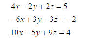
Example:
Solve the system of equations:

We represent these as the matrices

or as the single augmented matrix

This represents all the essential information about the system of equations in one place,
without the repetition of the variable names, so we can work with it instead. Augmented
matrices, therefore, are really just the original system written another way, and the
operations we do on each row are the same types of operations we’d do on each original
equation.

Recall that when we’re solving systems of equations using elimination we do it by adding
multiples of one equation to another to eliminate a variable.

The row operations we are allowed to do correspond to what we would do to the system
of linear equations, except now we don’t have to worry about x, y and z.

The allowed row operations are these.
• Multiply a row by a constant
• Add multiples of one row to another.
• Swap any two rows.

There are two methods, which differ only in their stopping point. Both will lead to the
same answer. The first is Gaussian elimination, which applies row operations until the
left-hand side of the augmented matrix is upper triangular. Then, the equations are
rewritten out and solved by back-substitution.

Your calculator has this – it’s called ref() which stands for row echelon form.

The gauss-jordan method goes a bit further until there is an identity matrix on the left
hand side. So it’ll look like

And then the solution is just x=a, y=b, z=c or (a,b,c).

Your calculator does the Gauss-jordan method using the command rref(). To use this,
you type the coefficients of the system into an augmented matrix (A say), and then do
rref(A). We’ll demonstrate in class.

Exercise 1: Once you know how to solve on your calculator, solve the system of
linear equations given by

Using both Gaussian elimination and gauss-jordan elimination.

When solving linear equations, we’re using the matrix as a big bag of numbers, rather
than using any properties of matrices themselves. In a sense, we don’t use an augmented
matrix as a real or proper matrix.

But matrices have interesting properties in their own right. We’ll do these now.

Matrix Addition
Only matrices of the same dimensions can be added. It works like this.

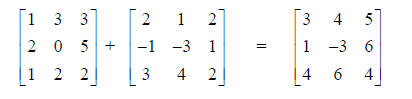
Note that the order doesn’t matter: A+B = B+A for any two matrices A and B.

Multiplication by a constant
This is also what you’d intuitively expect.

Multiplying two matrices
This is slightly less intuitive. Before looking at how it’s done, points to keep in mind are:
• It doesn’t work for every pair of matrices. Their dimensions must match in a
precise way.
• In general AB doesn’t equal BA.

First, the dimensions. The way it works is given in this example:

So the number of rows of the first matrix must match the number of columns of the
second. Think of chaining two dominos end to end.

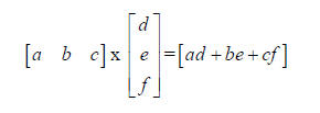
For the multiplication itself, the best way to explain it is to look at what happens for
some very small matrices (one row and one column respectively). For those who have
done trigonometry, a matrix with one row or one column is equivalent to a vector.

For larger matrices, multiply each row in the first one by each column in the second, just
like we did above. So the element in row 1, column 2 is got by multiplying the 1^st row by
the 2^nd column. In the example below, we have 2(-2) +1(4)+2(1)=2. Check the rest of the
matrix yourself as an exercise:

Note that the order matters in matrix multiplication – so that AB does not in general equal
BA. Even the dimensions may be different.

The Identity Matrix
Look at this example (and check the multiplication):

Note that the result is the same as the matrix we started with. The matrix

is a 3x3 identity matrix, and any 3x3 matrix when multiplied by it will give the same
result.

In general, the identity matrix is a square matrix with 1’s running along the diagonal, and
0’s everywhere else.

The transpose of a matrix
To get the transpose just swap the rows and columns. The transpose of a matrix A is
denoted by A^T.

A matrix is symmetric if it is identical to it’s transpose. Only square matrices can be
symmetric. For example (check this yourself):

Matrix Inverses
For a matrix A, if there is another matrix with the property that AB=I, the identity matrix,
then B is the inverse of A. Only a square matrix can have an inverse, and not all do.

Finding the inverse:
Example: to find the inverse of

Start with the augmented matrix:

And transform using row operations (if possible – if you can’t complete the
transformations the matrix has no inverse) until you have:

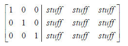
The matrix on the right hand side full of stuff is the inverse. Note that this is just like
gauss-jordan elimination, except with more stuff on the right hand side. So one way of
finding the inverse of a matrix on you calculator is to put it in an augmented matrix with
the identity matrix and use rref(). An easier way is just to type A^-1.

Exercise 2: For the Matrices

Find
a. AC
b. A-2B
c. (A-2B) C
d. A^-1